


Raman, Photoluminescence, and PLIM Imaging Using the RMS1000 Confocal Microscope
Key Points
- The ability to perform multiple complementary spectroscopic imaging techniques on a single sample is advantageous.
- Lifetime imaging is complementary to spectral photoluminescence and Raman because it provides information about the microenvironment of the sample.
- The RMS1000 Confocal Raman Microscope is capable of performing all three imaging techniques in one software package.
Introduction
In confocal microscopy, it is advantageous to combine multiple complementary spectroscopic techniques to maximise the information generated from a single sample. Two confocal spectroscopic techniques that are widely used are Raman and photoluminescence (PL) imaging, which provide information on the vibrational and electronic energy levels of the sample by reading out wavelength-dependent spectra.1 Both techniques can be performed on a confocal Raman microscope equipped with a continuous wave (CW) laser and a charge-coupled device (CCD) detector.
Another powerful imaging technique is fluorescence lifetime imaging (FLIM) or phosphorescence lifetime imaging (PLIM). In FLIM/PLIM, the variation in fluorescence or phosphorescence lifetime across a sample is imaged.2 Lifetime imaging can be used to determine chemical changes in the microenvironment of fluorophores/phosphors, detect conformational changes, and characterise properties like charge carrier efficiency in semiconductor materials and autofluorescence in tissue. Additionally, unlike intensity, the lifetime is independent of fluorophore/phosphor concentration, and it can be used to discriminate between materials that have overlapping emission peaks. Since FLIM/PLIM is a time-resolved method, it requires a pulsed excitation source, a photon-counting lifetime detector, and photon-counting electronics. 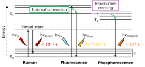
Figure 1. Jablonski diagram showing the energy transitions and relative timeframes of Raman scattering, fluorescence, and phosphorescence.
This Technical Note demonstrates how the RMS1000 Confocal Raman Microscope can be used to perform Raman, PL, and PLIM imaging of a sample all within a single software package. The integration of these three imaging techniques into the RMS1000 makes it ideal for both the analysis of multiple sample types and dedicated, in-depth studies of single samples.
Materials and Methods
Two photoluminescent rare-earth phosphors with different chemical structures and optical properties were mixed and deposited onto a calcium fluoride disk for spectroscopic imaging. Raman, spectral PL, and PLIM measurements were then performed on microparticles of the two phosphors using an RMS1000 Confocal Raman Microscope, Figure 2.
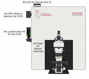
Figure 2. RMS1000 Confocal Raman Microscope setup used for Raman, spectral PL, and FLIM imaging.
The schematic in Figure 2 shows how the RMS1000 was configured for each imaging mode. For spectral PL and PLIM measurements, an externally coupled HPL-405 picosecond pulsed diode laser was used. For spectral PL the laser was operated at 80 MHz and used as a quasi-CW excitation source and the resulting PL emissions were detected using a back-illuminated charge-coupled device (BI-CCD) camera. For PLIM measurements, the HPL-405 laser was used at 10 kHz along with fluorescence and phosphorescence lifetime electronics capable of time-correlated single photon counting (TCSPC) and multichannel scaling (MCS), and a High-Speed photomultiplier tube (PMT) lifetime detector. For Raman measurements, the system was equipped with an internal 785 nm CW laser and the BI-CCD. The different excitation sources and detectors needed for each mode are summarised in Table 1. The three imaging modes were performed, and the necessary optical components for each mode were selected and changed, using Ramacle® software.
Table 1. Summary of the excitation source and detector needed for each imaging mode.
| Imaging Mode | Laser | Detector |
|---|---|---|
| PL Spectral | CW or pulsed (quasi-CW) | CCD |
| PLIM | Pulsed | PMT |
| Raman | CW | CCD |
Darkfield Microscopy
An area containing microparticles of the two phosphors was identified using darkfield imaging, Figure 3. The particles, labelled phosphor 1 and phosphor 2, were visually distinguishable under the microscope because they produced green and orange PL under white light illumination, respectively. This area of the sample encompassing the two particles was then analysed using PL, PLIM, and Raman.
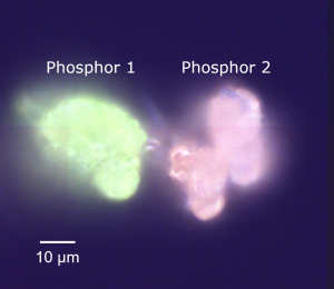
Figure 3. Darkfield image of phosphors 1 and 2.
Photoluminescence
The first spectroscopic technique used to analyse the sample was spectral PL imaging, Figure 4. The PL spectral image shows spectral intensity analyses for phosphors 1 and 2, which had peak emission wavelengths of 549 nm and 640 nm, respectively. 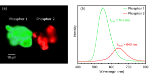
Figure 4. (a) PL image and (b) spectra of phosphors 1 and 2.
PLIM
Next, PLIM imaging was performed on the sample. Since the two particles produced PL spectra with different emission bands, the wavelength at which the two bands intersected (620 nm) was selected for lifetime measurements. The excitation rate was set to 10 kHz and the electronics module was set to record decays in MCS mode. The PLIM image and corresponding decays in Figure 5 show that the lifetimes of phosphors 1 and 2 were approximately 1.1 μs and 0.7 μs, respectively. Therefore, as well as distinguishing samples by their PL emission wavelengths, the RMS1000 can also be used to discriminate between them by their lifetimes.
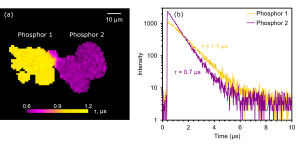
Figure 5. (a) PLIM image and (b) decays of phosphors 1 and 2.
Raman
Finally, to discriminate between the two phosphors by their chemical structures, they were imaged using Raman spectroscopy, Figure 6. Since the two phosphors exhibited PL at 549 nm and 640 nm, the 785 nm laser was selected to acquire the Raman image. This ensured that the resulting spectra were free from fluorescent backgrounds. 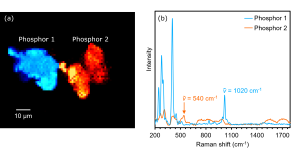
Figure 6. (a) Raman image and (b) spectra of phosphors 1 and 2.
The Raman image and corresponding spectra in Figure 6 show that the two phosphors exhibited unique vibrational spectra and hence had different chemical structures. The image of phosphors 1 and 2 was built by overlaying the intensity of the Raman bands at 1020 cm-1 and 540 cm-1.
Conclusion
Using the RMS1000 Confocal Raman Microscope, spectral PL, PLIM, and Raman imaging were used sequentially to thoroughly characterise and discriminate between two distinct phosphor microparticles, Figure 7. These techniques provide complementary information and are therefore useful for gaining substantial amounts of information and a cohesive understanding of samples under investigation.
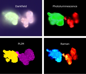
Figure 7. Darkfield, PL, PLIM, and Raman images of phosphor 1 and 2 microparticles.
