


What is Fluorescence Lifetime?
What is Fluorescence Lifetime?
Fluorescence lifetime is an important photophysical parameter that provides insight into the energy relaxation and dynamics of the species under study, such as energy transfer between molecular states, molecular rotation, and dynamic quenching.
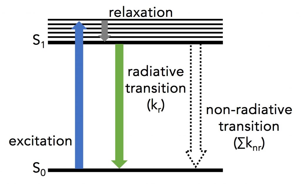
Figure 1: Simplified Jablonski diagram of a single molecule undergoing excitation and relaxation.1
Figure 1 shows a single molecule’s transition from its ground electronic energy level (S0) to the upper vibrational states of the first excited electronic energy level (S1) after light absorption (blue arrow). From there, the molecule rapidly relaxes non-radiatively (no photon emission) to the vibrational ground state of the S1 through vibrational relaxation (grey arrow). The molecule then returns to S0 either radiatively by emitting a photon (green arrow) or non-radiatively (dashed arrow). Kr and ∑knr are the radiative transition rate constant and the sum of non-radiative transition rate constants, respectively, that describe the depopulation of the molecule’s excited state.
For the molecule described in Figure 1, the fluorescence lifetime (τ) is mathematically defined as:1
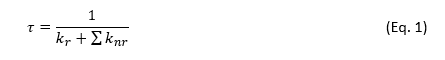
On a molecular level, τ corresponds to the average time a molecule spends in the excited state before returning to the ground state.1–3 Fluorescence is a random process and few individual molecules will emit exactly at t=τ; but across a large population of molecules, τ will be the average.
τ can be experimentally determined by exciting the population of molecules with a short excitation pulse (from a laser, LED or flashlamp) and recording the fluorescence intensity decay (Figure 2a).
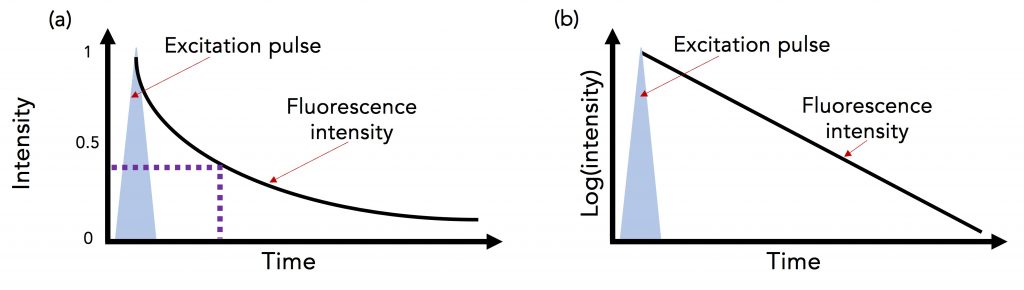
Figure 2 (a) Fluorescence intensity decay following a short excitation pulse on a (a) linear and (b) logarithmic intensity scale.3
For a population of molecules with a single lifetime τ, the intensity decay follows a single exponential decay model:
![]()
where t is the time from excitation and I0 is the initial intensity.1 τ is the time it takes the intensity to decrease to 1/e (=0.368) of its initial value. Fluorescence intensity decays are often plotted on a logarithmic intensity scale as log(I(t)) versus time (t), as shown in Figure 2b, which is a straight line for a single lifetime decay.
The fluorescence lifetime can be estimated from the measured decay using the time it takes the intensity to decrease to 1/e. However, it is more accurate to fit the intensity decay with a single exponential decay model to extract the lifetime using least squares fitting. Many samples exhibit fluorescence decays that are more complex than this example and exhibit multi-exponential or non-exponential behaviour and these must be analysed using more complex models.
More information on how to extract lifetimes from more complex fluorescence decays can be found in our next article: “Measuring Fluorescence Lifetimes”.
References
- J. R. Lakowicz, Principles of Fluorescence Spectroscopy. 3rd edition, Springer US, 2006. DOI: 10.1007/978-0-387-46312-4.
- B. Valeur, M. N. Berberan-Santos, Molecular Fluorescence: Principles and Applications. Wiley-VCH Verlag GmbH & Co. KGaA, 2012. DOI: 10.1002/9783527650002
- D. M. Jameson, Introduction to Fluorescence. CRC Press, 2014. DOI: 10.1201/b16502
