


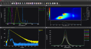
Figure 1: Fluoracle Software interface
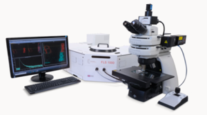
Fluoracle® is a comprehensive, user-friendly software package for instrument control and data analysis at the heart of all Edinburgh Instruments fluorescence spectrometers. It provides the user with complete control of the instrument as well as third-party accessories irrespective of configuration.
Fluoracle is Windows compatible and features intuitive setup menus, live signal display, easy switching between measurement modes and user-friendly analysis wizards. This guarantees ease of use in the operation of a modular and potentially complex spectrometer. Common measurement routines can be saved as method files to allow previous experiments to be easily repeated.
Light sources, detectors, complex sample holders (microplate reader, XY sample stages, titrator) and cooler options (thermostated sample holders and cryostats) are fully software controlled. Fluorescence Lifetime Imaging Microscopy (FLIM) acquisition and analysis are included in Fluoracle with a MicroPL upgrade.
Fluoracle offers the FAST add-on for the advanced analysis of fluorescence and phosphorescence decay kinetics.
Besides standard excitation and emission spectra, Fluoracle can perform synchronous scans, excitation-emission maps (EEMs), and kinetic scans at a single or multiple wavelengths. The example shows an EEM acquired with a camera, which provides maximum acquisition speed acquiring a full emission spectrum in a single shot.
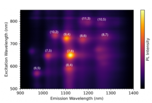
Figure 1: EEM of single-wall carbon nanotubes in aqueous surfactant solution, acquired in FLS1000 with Xenon lamp excitation and InGaAs NIR camera. Identified nanotube structures shown in map.
Temperature-dependent measurements and photoluminescence quantum yield are possible with suitable accessories. Cryostats, TE-cooled cuvette holders, and external cryostages for microscopes are all compatible and controlled by Fluoracle.
Figure 2: Temperature-dependent photoluminescence spectrum of a halide perovskite measured in an FLS1000 with a software-controlled cryostat.
Using Batch measurement mode, customised series of scans can be set for a sample and measured automatically without the presence of the user. Loops and delays between scans can be programmed easily. The batch measurements (protocols) can be saved and loaded for future use. Communication with almost any external accessory is possible via a USB COM port command interface.
Steady state fluorescence anisotropy, singlet oxygen detection, chromaticity measurements, upconversion photoluminescence, electroluminescence, water quality assessments, absorption, and much more.
Acquisition and analysis of time-resolved fluorescence is easy with the FLS1000. Fluoracle offers easy measurement wizards for time-correlated single photon counting (TCSPC), as well as analysis tools for exponential decay fitting.
The analysis routine provided is based on the Marquardt-Levenberg algorithm. Up to four exponential decay components can be fitted and additional fit quality parameters are available for quality assessment, such as autocorrelation functions, the Durbin-Watson parameter and standard deviations.
Figure 1: Results of a reconvolution fit with tests against three multi-exponential decay models. Experimental data (green), IRF (blue), and fitted curve (red). Residuals for one-exponential and two-exponential fits are shown to illustrate the improvement in fit quality.
With Time-Resolved Emission Spectra (TRES), a family of decay curves is automatically acquired as a function of wavelength. The data slicing option in Fluoracle allows to easily convert the family of decay curves into a family of time-resolved emission spectra.
Figure 2: TRES and time-resolved emission spectra from norharmane in ethanol, 0 – 200 ns, acquired with EPLED-280 excitation in FLS1000.
Time-resolved anisotropy, monomer-excimer kinetics, solvent relaxation dynamics and much more.
The photoluminescence emission lifetime of metal halide hybrids extends over a large time range from nanoseconds to milliseconds. In this case the method of choice for time-resolved measurements is the Multichannel Scaling (MCS), which provides speed of measurement with photon-counting sensitivity.
In the example, two TRES profiles of Tris SbMnCl were measured, the first focusing on the 0-20 µs time range with a time-resolution of 50 ns (a & b); and a second over a time range of 50 ms with a lower time-resolution of 10 µs (c & d) to capture the long timescale behaviour.
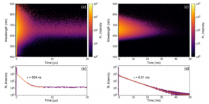
Figure 1: TRES of Tris SbMnCl acquired over (a) a 20 µs time range and (b) a 50 ms time range. Extracted decays at λem = 650 nm are shown in panels (b) & (d).
A gated PMT detector may be used in MCS mode to discriminate between fluorescence and phosphorescence. Gating the detector allows measuring weak phosphorescence without saturating it with fluorescence light.
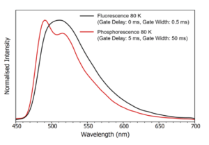
Figure 2: Fluorescence and phosphorescence spectra of a thermally activated delayed fluorescence (TADF) material, CzDBA, acquired with a gated PMT and VPL-375 source in MCS mode.
Time-resolved singlet oxygen measurements, time-resolved FRET measurements and much more.
The QYPro Integrating Sphere enables easy measurements of absolute photoluminescence quantum yield (PLQY) in the visible and NIR range. This method is more accurate than the relative QY approach, does not require a QY standard and is readily applicable to liquids, films and powders.
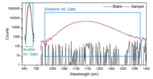
Figure 1: Absolute PLQY measurement of PbS quantum dots in tetrachloroethylene. The range integrated for the scattering peak is highlighted in teal, and the integration range for the emission peak is highlighted in blue.
Reflectance and absorbance of solids and powders are easily acquired in an FLS1000 with QYPro integrating sphere. Synchronous scans of the sample and reference are converted into reflectance of absorbance in the Fluoracle software.
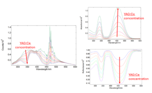
Figure 2: Synchronous scans of YAG:Ce phosphor in BaSO4 at various concentrations, absorbance and reflectance results.
The FLS1000 can be equipped with double monochromators on excitation and emission arms. Double monochromators are recommended for highly scattering, low emissive samples as they improve the system’s stray light suppression and increase the signal-to-noise ratio. A double monochromator in the emission arm allows for up to three detectors mounted simultaneously with software-based selection; two detectors can be fitted after the double monochromator and one after the first of the two monochromators.
If further detectors are required, the system can be configured in a T-geometry by the addition of a separate emission monochromator. This configuration can also be useful to provide a digital detection arm and an analogue detection arm.
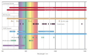
450 W continuous wavelength lamps for steady state measurements. The excitation range is typically 230 nm to >1700 nm. Ozone generating lamps may be used to increase the lower range to 180 nm.
μF1 and μF2: 5 W or 60 W pulsed xenon microsecond flashlamps producing short microsecond pulses for phosphorescence decay measurements. The excitation range is typically 230 nm to 1000 nm.
We manufacture a range of picosecond pulsed laser diodes (EPL Series, HPL Series) and pulsed LEDs (EPLED Series) for Time Correlated Single Photon Counting (TCSPC) measurements, as well as variable pulsed lasers and diodes (VPL Series, VPLED Series) for Multi-Channel Scaling (MCS). Diodes are available over the UV-VIS spectrum starting at 250 nm and are pre-set with a range of repetition frequencies but can also be pulsed externally. The driver electronics are built into the light sources, eliminating the need for additional driver boxes and feature true “plug-and-play” usability.
Visit our Pulsed Lasers and LEDs page for full details.
AGILE® is a supercontinuum laser providing picosecond pulses with variable kHz to MHz repetition rates. It couples to the FLS1000 for continuous wavelength tuning from <400 nm to >2000 nm. AGILE is the ideal source for TCSPC with a wide range of excitation wavelengths and is also compatible with MCS operation.
Find out more about AGILE supercontinuum laser.
An ultrafast nanosecond flashlamp is available for time-resolved fluorescence studies in the range of 100 ps – 50 μs. The excitation range is tuneable and gas dependent (UV-Visible).
Various continuous wave lasers for use with the FLS series are available. Some CW laser sources may also be pulsed by the spectrometer to allow, for example, upconversion decays with 808 nm and 980 nm excitation to be measured.
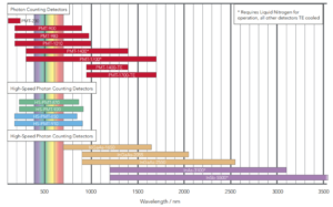
Single photon counting detectors comprise a single photon counting photomultiplier with an optimised dynode chain, mounted in a light-tight cooled or un-cooled housing.
The following PMTs are available: Standard PMTs up to 1010 nm, High speed PMTs up to 850 nm, MCP-PMT up to 850 nm, NIR-PMTs up to 1700 nm and gated PMTs.
A high-speed hybrid photodetector covering the visible range is available.
Analogue detectors are used either for high light level applications with the requirement for high dynamic range, or as alternative detectors in spectral ranges where photomultipliers are unavailable. Depending on the required application, the analogue detectors come in a variety of housings with a variety of cooling options. Analogue detectors find application to extend the spectral coverage into the NIR to 5.5 µm.
We offer detector assemblies that are supplied for steady state fluorescence, time-resolved fluorescence and/or time-resolved phosphorescence applications.
The QYPro integrating sphere is an additional accessory to the FLS1000 for the measurement of photoluminescence quantum yield (PLQY) and spectral reflectance properties. The QYPro is mounted within the FLS1000 sample chamber ensuring no loss of signal from external coupling methods.
The large internal diameter of the sphere, coupled with our proprietary calibration procedure, ensures accurate results from the UV to the NIR. The QYPro’s powered external sample loading mechanism makes sample exchange quick and easy. It also reduces the risk of contamination, which is vital for maintaining accurate results over the lifetime of your integrating sphere. 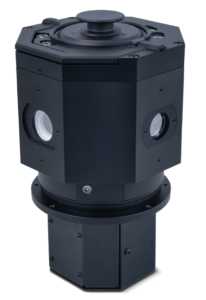
The QYPro is our most flexible integrating sphere to date, with interchangeable excitation ports allowing you to measure your samples with our multitude of FLS1000 system geometries and excitation sources. The standard photoluminescence sample accessory kit provides sample mounting options for solutions, thin films, powders and bulk materials. The QYPro also comes with a gas purging kit as standard allowing you to study air-sensitive samples with ease.
Data analysis is quick and easy using the PLQY wizard of the Fluoracle® software.
You can view all our QYPro focussed videos on our YouTube Channel: QYPro Videos.
The MicroPL upgrade allows spectral and time-resolved photoluminescence measurements of samples in the microscopic scale. The FLS1000 is upgraded with a microscope so you can finely tune both the excitation light (illumination) and the detected emission, using widefield or point excitation.
The microscope can be supplied as either an upright and inverted microscope. Imaging cameras are available spanning the spectrum from the visible to the near-infrared, up to 1700 nm. Excitation can be provided by halogen lamps (wide field excitation), picosecond pulsed diode lasers and pulsed LEDs, supercontinuum sources and Nd:YAG lasers (lasers provide point source illumination).
Steady state emission spectra and fluorescence lifetime measurements can be obtained from specific spots on your sample, when using appropriate lasers. Lasers can achieve a spot size of ~2 μm (objective dependent). The optional FLIM add-on includes a computer-controlled XYZ stage and unlocks special features in the Fluoracle software including advanced analysis options for maps, such as multi-component decay fitting algorithms.
Download the MicroPL datasheet for full details.
The XS1 X-ray Radioluminescence Chamber is an external sample chamber housing X-ray sources (pulsed and/or CW) for time-resolved and steady-state X-Ray luminescence spectroscopy. The X-ray induced luminescence is collected by a liquid light guide which delivers the light to the FLS1000 spectrometer for detection.
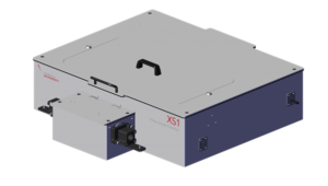
Sample holders for cuvettes, slides and powders are included. The pulsed X-ray source must be optically excited with a picosecond or nanosecond laser (EPL or HPL series) to generate X-ray pulses which can be as fast as 150 ps (laser dependent), enabling the measurement of decays in the sub-nanosecond range.
The Circularly Polarised Luminesence (CPL) upgrade for the FLS1000 provides CPL spectra from chiral samples which emit circularly polarised light. The upgrade comprises a photoelastic modulator acting as an oscillating quarter-wave plate which, together with an emission polariser, selectively transmits left or right circularly polarised light.
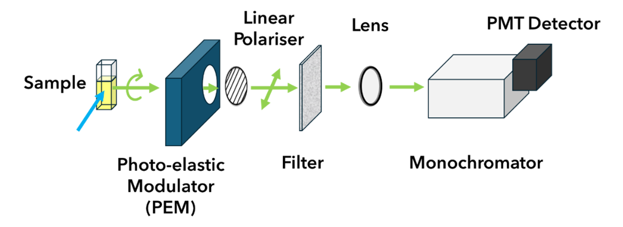
The results are expressed as emission circular intensity differential (ECID), i.e. the difference in intensity of the left and right circularly polarised components; and as the dissymmetry factor glum.
CPL spectroscopy is a valuable addition to the FLS1000 spectrometer for studying lanthanoid complexes, materials for 3D displays, security applications, as well as biosensors and pharmaceutical compounds.
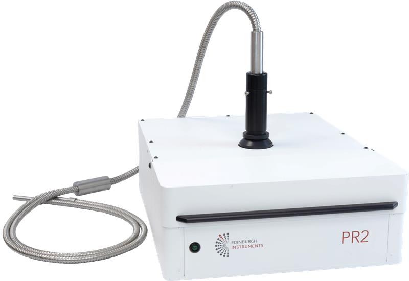
The PR2 microplate reader is an external module that is attached to the FLS1000 to perform spectral or time-resolved PL measurements on microplates. It supports user-defined microplate configurations up to 384 wells. The plate reader module is coupled to the FLS1000 by means of a bifurcated optical fibre. The control of the module is fully automated from the Fluoracle software. The spectral range supported depends on spectrometer and bifurcated fibre assembly configuration.