TRES (time-resolved emission spectra) is a type of photoluminescence measurement where lifetime decays for a sample are collected at a range of emission wavelengths (Figure 1a). The decays may be represented as a function of wavelength in a colour plot (Figure 1b). By integrating decays over a fixed time period, the dataset is sliced, resulting in a spectrum at that time period; the time-resolved emission spectrum (Figure 1c).1
This is achieved by using a pulsed excitation source to excite the sample and collecting emission decays for a range of emission wavelengths by Time-Correlated Single Photon Counting (TCSPC) or Multichannel Scaling (MCS).
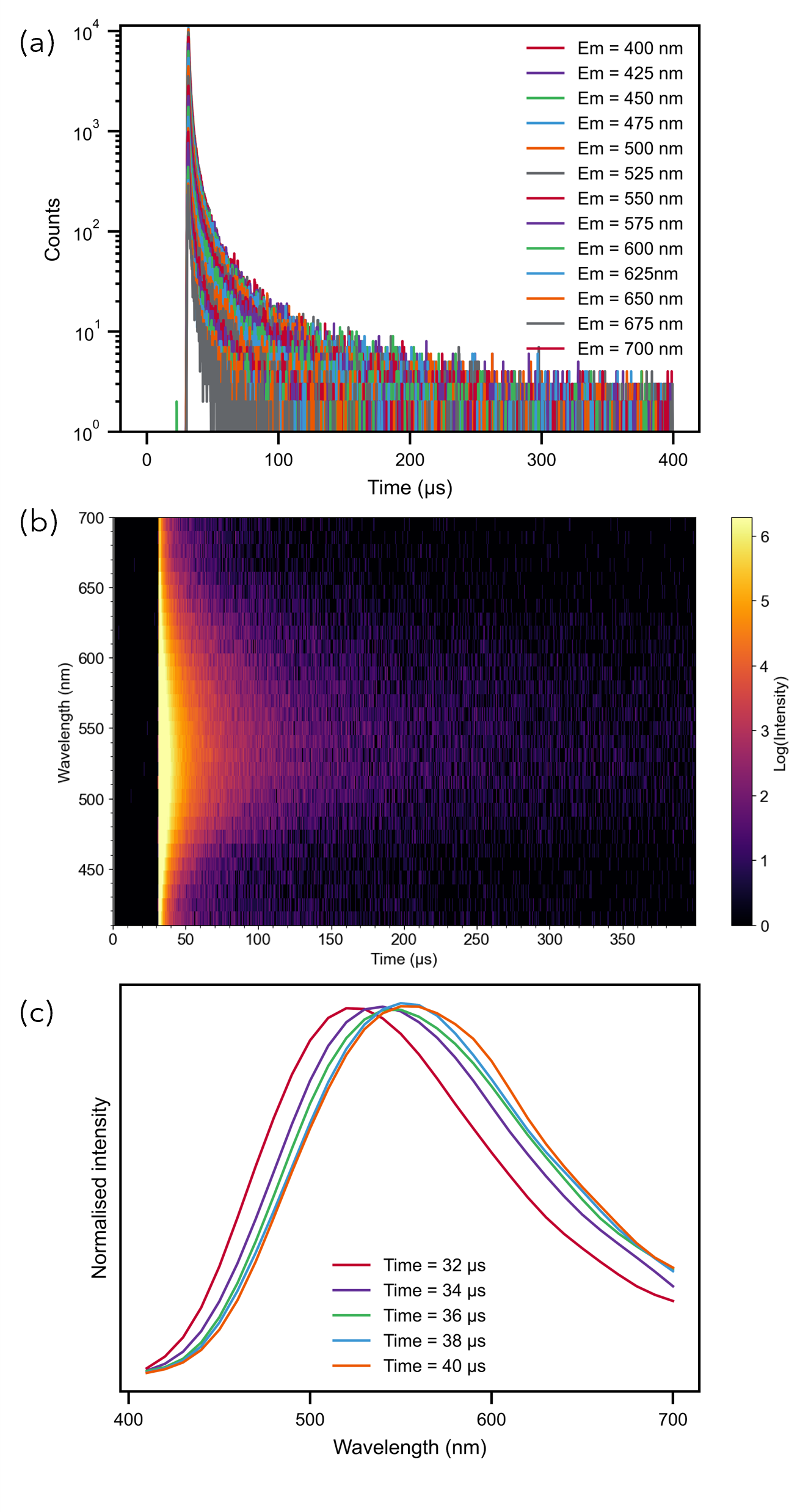
Figure 1: An example TRES of a Cu-N-TiO2 sample (a) 2D plot shows the decays collected at a range of emission wavelengths. (b) Decays represented as a colour plot as a function of emission wavelength (c) TRES for a range of time slices.
An analogous technique is TRES excitation, where lifetime decays are collected with a range of excitation wavelengths. For this, a pulsed wavelength-tunable source is required.
This technique is useful when a sample has several emission bands with different lifetimes. This could occur in several luminescent samples such as:
TRES can give information on the homogeneity of the sample, the mechanism of emission of the sample, and may be used to separate individual spectra of overlapping emission bands. We will outline some examples of these below:
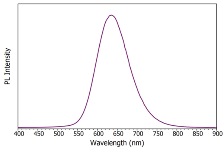
Figure 2: Emission spectrum of a Tris SbMnCl sample.
In this example, the emission spectrum of a sample of Tris SbMnCl, shows a single peak, but could there be other bands hidden underneath?
Two TRES colour plots collected at a 20 µs and 50 ms time range show that there are 3 components to the photoluminescence decay with different time scales: a short ns component, an intermediate µs component, and a longer, ms component (Figure 3a, b). We can see this more easily when we look at the extracted decays for the two time ranges at 650 nm (Figure 3c, d).
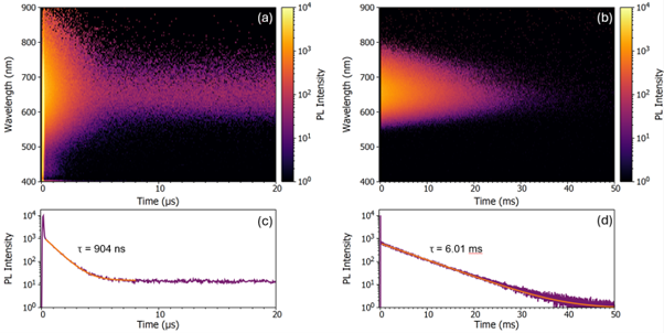
Figure 3: TRES colour plots of Tris SbMnCl collected at (a) 20 µs and (b) 50 ms timescales. Extracted emission decays at 650 nm at (c) 20 µs and (d) 50 ms timescales.
By integration of the decay curves, the plot can then be sliced to reveal individual spectra at the different time periods. Normalising the resulting spectra allows us to observe three distinct bands (Figure 4a). The ns and µs components may be assigned to the respective fluorescence and phosphorescence emission of Sb in these types of materials. The ms component can be assigned to Mn centres in Tris SbMnCl as it is also observed in its precursor, Tris MnCl (with no Sb doping). When we look at the relative intensity of the spectra (Figure 4b), we can see that Mn is the dominant emitter, which is why it dwarfs the other two bands in the emission spectrum.
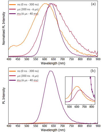
Figure 4: Extracted emission spectra of the ns, µs, and ms channels of Tris SbMnCl with (a) normalised intensities, and (b) relative intensities.
TADF is a process where certain materials can undergo reverse intersystem crossing (RISC) from a triplet state excited state (T1), back to a singlet excited state (S1) and then to the singlet ground state (S0), emitting a photon. This process is of great importance for achieving highly efficient organic light-emitting diodes (OLEDs) without the use of expensive heavy metals. To learn more about this process, read our spectral school on TADF.
Decays of TADF emitters will have a short lifetime component, corresponding to the S1 → S0 transition, and a long lifetime component, corresponding to the T1 → S1 → S0 transition via RISC. But how can you tell whether the long lifetime component is due to TADF, or simply a phosphorescent T1 → S0 transition?
TRES can help reveal the answer.
After collecting the TRES plot, we can take slices at the two time ranges to reveal their spectra (Figure 5a). If the spectrum for the prompt fluorescence matches the spectrum for the delayed fluorescence, then it is most likely proceeding via TADF, as both bands arise from an S1 → S0 transition. If it doesn’t, then it is likely that the longer lifetime component is due to a different mechanism, such as phosphorescence, which is not as useful in the development of OLEDs.
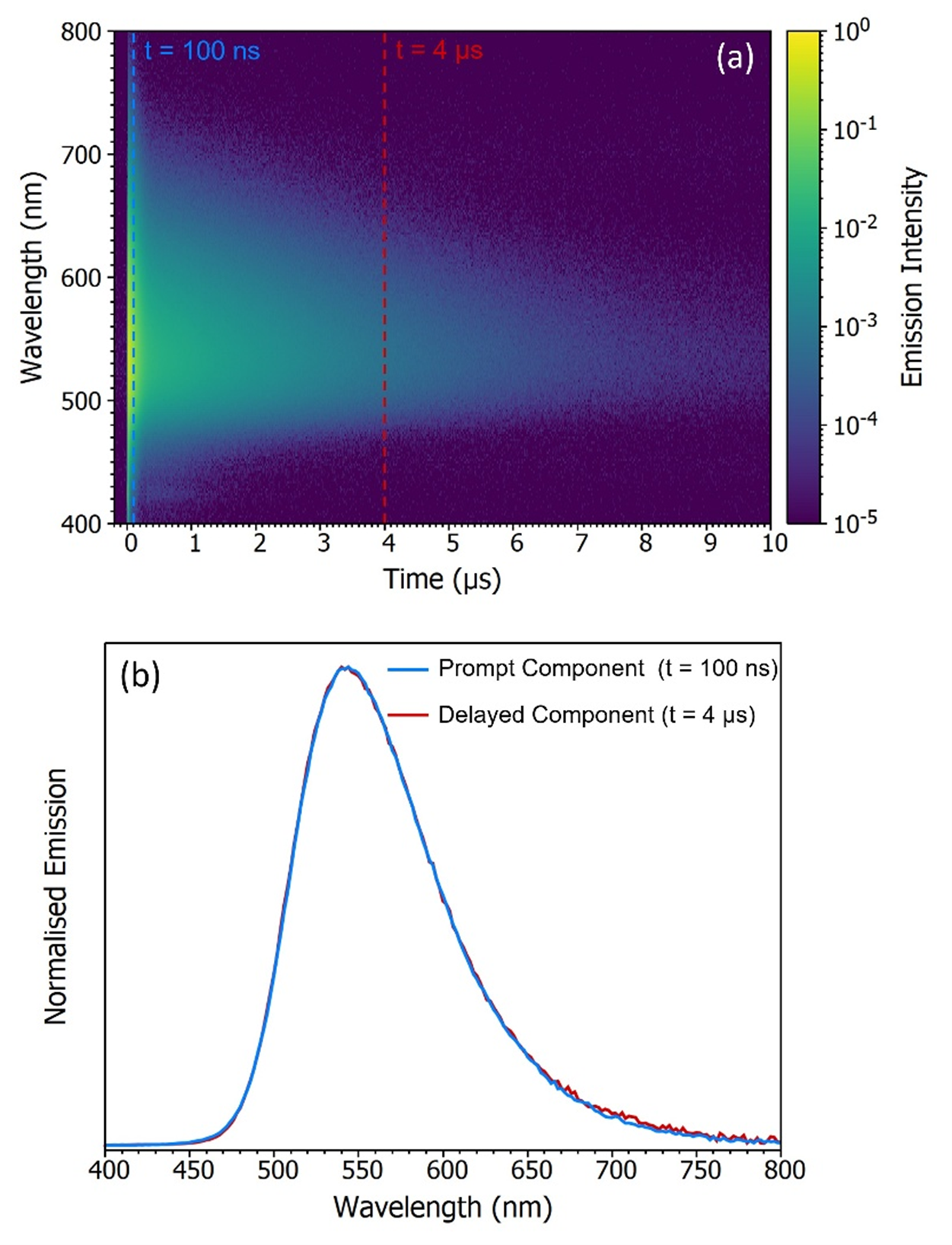
Figure 5: (a) TRES colour plot of a TADF material (b) TRES slices of the prompt and delayed emission.
In this case, the spectra of the prompt and delayed component match which indicates that this material is indeed undergoing TADF (Figure 5b).
TRES may also be used to characterise defects or imperfections that influence how a material emits light. In this example, quantum dots made with the semiconductor indium phosphide with a zinc sulfide coating (InP/ZnS) were analysed. InP quantum dots alone are not emissive due to non-radiative recombination at trap sites on the particle surface. As such, they are often coated with a ZnS semiconductor layer which passivates the traps and enhances quantum yield.
But how can we be sure that the traps have been fully passivated or not?
Figure 6: TRES colour plot of InP/ZnS quantum dots.
TRES can help us answer this question as trap emission and semiconductor band edge emission occur on different timescales and at different wavelengths.
From the TRES colour plot, we can see that as emission wavelength increases, there is an emissive tail with a long lifetime (Figure 6). Extracting and fitting decays at 620 nm and 775 nm reveals they exhibit intensity-weighted average lifetimes of 31.2 ns and 348 ns respectively. As the tail region around 775 nm has a lifetime a magnitude greater than the band edge at 620 nm, this suggests the presence of traps in the dots, and incomplete passivation of InP by ZnS. The reason for this could be that the ZnS layer is too thin, and the synthesis could be optimised to address this.
TRES is a powerful technique in photoluminescence spectroscopy. It can reveal hidden emission bands, characterise emission mechanisms, as well as provide information regarding the electronic and physical structures of optical materials.
At Edinburgh Instruments, TRES measurements are available for spectrometers with a monochromator, such as the FS5 and FLS1000 photoluminescence spectrometers. If you would like to find out more about our products and how they could aid your spectroscopic analysis, please get in touch with our friendly team by completing this form.