Time-Correlated Single Photon Counting (TCSPC) outperforms all other techniques in sensitivity, precision, dynamic range, and data accuracy. Complex fluorescence decays can be fitted by reconvolution or tail fitting to identify multiple lifetime components.
This Spectral School tutorial is a deep dive into some of the more advanced TCSPC concepts. An introduction to TCSPC can be found at What is Time-Correlated Single Photon Counting?
TCSPC is a time domain technique. Data is accumulated, presented, and analysed in a format showing signal intensity versus time, usually in picoseconds, nanoseconds, or microseconds. Exponential component analysis is used to fit the data to a user selectable number of components which can describe the decay. The fit is evaluated by examination of the residuals and the χ2 value. These components describe the fluorescence lifetimes of the emissive populations present in the sample. The presence of multi-exponential or more complex decay kinetics can be seen when viewed in a semi-logarithmic scale (Figure 1).

Figure 1. A three exponential component decay curve. On a semi-logarithmic scale, a multi-exponential decay appears to be curved. The residuals of fitting and the χ2 value confirm that this decay curve is best described by three exponential components. Decays recorded on an FLS1000 using a Ti:Sapphire excitation source and an MCP-PMT detector.
TCSPC counts single photon events, therefore detection is at the quantum limit. The technique requires an excitation source with a high repetition rate, pulsed output. As the process of capturing a single photon is repeated several thousand or even a million times per second, a sufficiently high number of single photons is processed for the resulting fluorescence lifetime measurement.
Only one photon is processed at a time, so the light pulses required for sample excitation have low pulse energy. This causes minimal sample degradation and avoids many non-linear effects.
TCSPC covers lifetimes of over 7 orders of magnitude. Instrument response functions of less than 50 ps (5×10-11s) are obtained with a combination of the fastest detectors on the market (HS-HPD) and mode locked femtosecond lasers. Numerical reconvolution enables fluorescence lifetimes of less than 5 ps (5×10-12 s) to be recovered. The upper limit of the lifetime range is 50 ms (5×10⁻⁵s).
Time Correlated Single Photon Counting (TCSPC) is a counting technique, thus principally a digital technique rather than an analogue one. The only relevant data noise is the Poisson noise (or counting noise). The Poisson noise is well defined and is precisely the square-root of the data point. The fact that we know precisely the noise has big consequences for numerical data analysis, where each data point needs to be properly weighted.
TCSPC data obeys Poisson noise statistics. Poisson noise is not a constant noise that is added to each data point of the decay curve. The noise value of each data point is different and the square-root of the signal itself. In simple words big data values are “noisier” than smaller data values. Therefore, in TCSPC smaller data values can be better viewed and analysed than with analogue techniques. The reason why TCSPC data is generally demonstrated on a semi-logarithmic scale is the Poisson noise of the data.
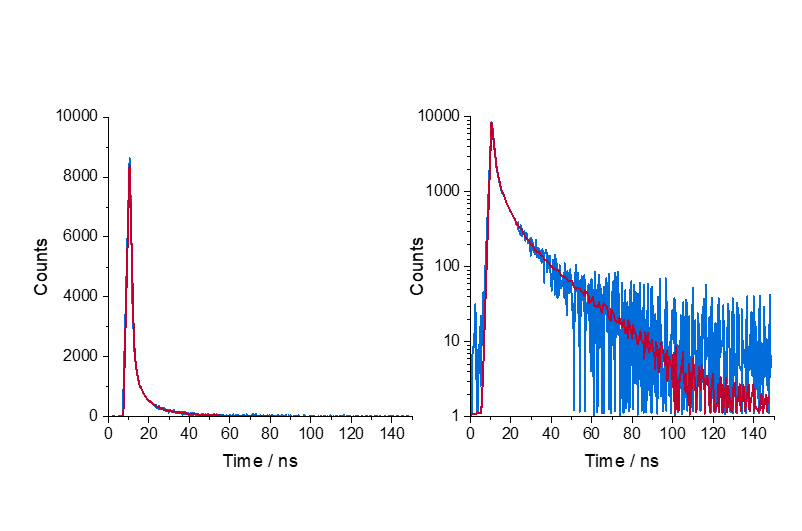
The dynamic range of a TCSPC measurement is typically 104:1, as a single photon can be observed as well as the signal maximum (typically 104). It can even be bigger if data are acquired beyond 10,000 counts at the maximum.

Figure 2. Typical fluorescence decay with Poisson noise (red) and Gaussian noise (blue) shown on a linear (left) and logarithmic scale (right). Poisson noise statistics allow for a greatly increased dynamic range.
TCSPC provides the highest time resolution among techniques using single photon detectors. The distinct advantage of TCSPC is that this technique does not use the analogue detector response to produce the instrumental response function (IRF). The jitter in the rising edge of analogue detectors dictates the width of the IRF. The rising edge jitter of photomultiplier detectors (the transit time spread) is typically only 10% of the analogue pulse.
TCSPC is (over a wide range) insensitive to fluctuations in pulse amplitudes of the excitation light source; to fluctuations of the detector output pulses and to background noise of the detector. For many detectors, the background (which also obeys Poisson statistics) is largely eliminated by a threshold allowing only pulses of a certain pulse amplitude to be processed (leading edge discrimination). The constant fraction discriminator evaluates the pulse’s temporal position by the fastest rise of the pulse. Thus, pulses of different pulse height amplitudes still start (or stop) the “clock” at the same time. Pulse height fluctuations either from light source instabilities or from the intrinsic pulse height fluctuation characteristics of photomultipliers are largely irrelevant.