Time-correlated single-photon counting (TCSPC) is the method of choice for quantifying fluorescence lifetimes. It can be used for the spectroscopic characterisation of a wide variety of solid, liquid, and gas samples, and when combined with optical microscopy it allows for fluorescence lifetime imaging (FLIM) to be performed.

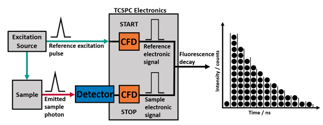
Figure 1. Simplified overview of TCSPC with two inputs (Reference START and Sample STOP) producing a histogram of timed events binned into channels split evenly across the time range.

Figure 2. Pulse collection in TCSPC where the START line is supplied from the excitation source and the STOP is connected to the sample emission. Where no STOP signal is received within the window, the electronics must reset before the next START pulse
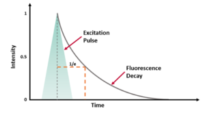
An example of a single exponential fluorescence decay acquired using TCSPC is shown in Figure 3. As well as the sample decay, the plot also includes the Instrument Response Function (IRF) which is characteristic of the specific measurement system, and a reconvolution fit of the decay to two components.

Figure 3. Fluorescence decay of a sample (blue) and the IRF (red) plotted on a logarithmic scale with the fitting of the data by revolution analysis (grey) and the residuals of this fit below (black).
TCSPC can be used to measure lifetimes as low as a few picoseconds up to hundreds of nanoseconds- over 7 orders of magnitude. At the lower limits of detection, the temporal response of the specific system, IRF, must be considered. The IRF is found by measuring the full width half maximum (FWHM) of a scattering solution at the excitation wavelength. This represents the shortest decay a system could resolve, as any fluorophore with a lifetime significantly shorter than the FWHMIRF will appear as the IRF. When recording decays on the order of magnitude of the IRF, reconvolution fitting should be used to extract the influence of the IRF on the shape of the decay function. The IRF will be affected by four components of the system: the pulse width of the excitation source used, the width response of the detector, the electronic jitter of the counting electronics, and the temporal dispersion through the emission monochromator. The response of the detector is usually the limiting factor in the sensitivity of a TCSPC system.
There must be sufficient time range to allow the fluorescence signal to decay down to the level of the background counts before the next counting cycle may begin as shown in Figure 3. Where this is not implemented, the decay will start to ‘wrap-around’ the window, distorting the peak of the next decay as it will appear to have arisen from the proceeding start event. In measurements with low sample count rates and high background and/or dark counts, the rising baseline will limit the dynamic range by masking the tail of the decay which leads to an underestimate of the lifetime.
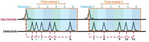
In TCSPC a maximum of one photon can be detected after each START pulse. In Figure 4 we can see that that three photons arrive within the first START window; but after the first photon is detected, the electronics cannot see any subsequent photons. Since faster photons will arrive at the detector first, the photon histogram will be distorted towards these faster arriving photons.

Figure 4. Illustration of pulse pile-up effect. Of three emitted photons in the first pulse period, only the first to arrive is seen by the electronics
This phenomenon is called pulse pile-up and would distort the measured fluorescence decay. To prevent pulse pile-up the STOP rate is limited to below 10 % of the START, to so that the statistical probability of two photons arriving in the same START window is negligibly small. This maximum STOP rate is suggested between 1 and 10 %,1–4 Edinburgh Instruments Fluoracle advises a maximum of 5 %. For instance, the repetition rate of a 100 kHz source would have recommended maximum count rate of 5,000 Hz.
The examples described here all show a system operating in the conventional Forward Mode. The drawback of Forward Mode is observed when using excitation sources with high repetition rates, like Ti:Sapphire lasers which can reach well over 50 MHz. This is because the time between START pulses is less than the time required to reset the electronics, known as the dead time. If START pulses arrive during the dead time the electronics will not start so higher START rates will not decrease the decay acquisition time and photosensitive samples will be more prone to bleaching due to increased exposure. Instead, the system may be operated at the rate of the emission pulses by using Reverse Mode. In Reverse Mode, an emitted photon from the sample is used to START counting, and the excitation laser pulse STOPS the counting. Starting the counting electronics from the receipt of an emitted photon means that the counting electronics will only be activated when there is a count to be recorded. Reverse Mode has great utility in FLIM applications, where a large area must be scanned, and the decays can be acquired as quickly as possible.
The main components of the TCSPC electronics are the Constant Fraction Discriminator (CFD), an electronic delay (Delay), the Time-to-Amplitude Converter (TAC), an amplifier (not shown), an Analogue-to-Digital Converter (ADC), and the digital memory (MEM) shown in Figure 5.

Figure 5. Schematic showing the main components of signal processing in TCSPC electronics.
START and STOP signals are received at the constant fraction discriminator (CFD) where the pulse must surpass the Threshold voltage. This eliminates low amplitude noise from being counted as a real signal. The zero crossing may be adjusted to tens of mV above or below zero to reduce the timing jitter due to irregular pulse height.3 This produces an electronic pulse which is independent of amplitude to be passed to the TAC. The STOP signal may be delayed to position it optimally in the recorded window so that the background counts can be viewed before the decay, and to confirm the emission drops back to the background level by the end of the window as shown in Figure 3.
The TAC starts ‘counting’ (gain) until a STOP signal (emitted photon) is received. If no signal is received in this time, the charge is dispersed to reset the TAC for the next cycle. When a signal is received, the amplitude which has accumulated in this time is passed to the amplitude to digital converter (ADC) and is binned to the appropriate channel, building up a histogram of time against counts. The resolution of the channels may be altered by selecting a shorter time range or increasing the number of channels.
The time window can be tuned to detect fluorophores on a time scale from 10 picoseconds to 8 microseconds depending on the system configuration.2 Longer photoluminescence decay times can be measured using Multi-Channel Scaling (MCS).
1 W. (Wolfgang) Becker, Advanced time-correlated single photon counting techniques, Springer, 2005.
2 J. R. Lakowicz, Principles of Fluorescence Spectroscopy Third Edition, 2010.
3 W. Becker, The bh TCSPC Handbook, 8th edn., 2019.
4 B. Valeur and M. N. Berberan-Santos, Molecular Fluorescence, Wiley-VCH, 2nd edn., 2012.
If you have enjoyed this blog, be sure to subscribe to our enewsletter and follow us on social media to keep up to date with the latest products news and updates.