A photoluminescent or fluorescent decay can be analysed to extract the lifetime(s). When fitting a decay, the sample’s underlying photophysical processes must be considered to help evaluate the appropriateness of the fitting. Here, we will explore the analysis of single, multi, and non-exponential decays using discrete component fitting in Fluoracle®. 

Excited State Populations

Time-Correlated Single-Photon Counting examines the rate of decay for excited state populations, [M*]. The decay in the concentration of excited state molecules, [M*], at time, t, can be written as:

Here, [M*]0 is the concentration of molecules in the excited state at time = 0. Time = 0 is equivalent to the arrival time of the excitation pulse in TCSPC fluorescence measurements. There are multiple competing deactivation processes, split into radiative and non-radiative pathways. The rate constants associated with these parameters are kr and knr, the rate constants for the radiative and sum of the non-radiative processes respectively. The term k may be introduced to signify the sum of all rate constants. 

However, we can’t directly measure the concentration of excited state molecules. Instead, a measurable parameter is the fluorescence intensity, I. The relationship between the fluorescence intensity at a time, t, and the decay in the fluorescence intensity is shown in Equation 2. 

where τ is the fluorescence lifetime. τ is defined in relation to the rate constants according to: 

How to Fit Single Exponentials Decays

The simplest fluorescence decays exhibit single exponential behaviour: 

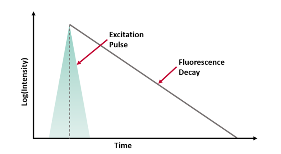
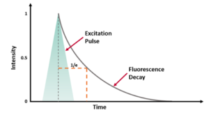
where t is time, τ is the fluorescence lifetime, and B is the pre-exponential factor. The fluorescence lifetime is defined as the time it takes the intensity to drop to 1/e (=0.368) of its initial value (Figure 1a). Fluorescence decays are most often shown on a logarithmic scale which gives a linear response for a single exponential decay (Figure 1b). 

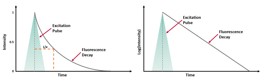
Figure 1. Representation of a fluorescence decay following a short excitation pulse on a (a) linear and (b) logarithmic scale.​1​ 

Fitting Methods

To extract components from a decay, it must be fitted to an appropriate function. There are two common methods of fitting TCSPC data, tail fitting and reconvolution fitting. Over multiple iterations, the parameters of lifetime and B-factor are varied to optimise the fit to the collected decay. 

When a sample has long fluorescence lifetimes, tail fitting can be used. This involves fitting from the peak of the decay without convolution with the Instrument Response Function (IRF).  

When studying short-lived excited state populations, iterative reconvolution is used. The theoretical decay function is convoluted with the measured IRF.  

Fitting Evaluation

The fit can be evaluated by calculation of the χ2. This function calculates the difference between the raw data points and the fitting points to quantify how well the data has been replicated. 

The difference between the measured fluorescence decay function, N(tk), and the calculated decay function, NC(tk), are evaluated across the number of data points, n. 

A χ2 value of 1 indicates that the system is replicated by the fit. A value above 1.2 can indicate that the system is not well described by the fit. The bounds for an acceptable χ2 will vary on the experimental system, specifically with the noise associated with it. Good practice should include measurement of a well-established single component fluorophore prior to sample measurement to establish the achievable sensitivity of the system. 

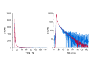
The fluorescent dye 9-aminoacridine (9AA) in solution is a classic example of single exponential behaviour. The fluorescence decay of 9AA dye measured using TCSPC is shown in Figure 2.  

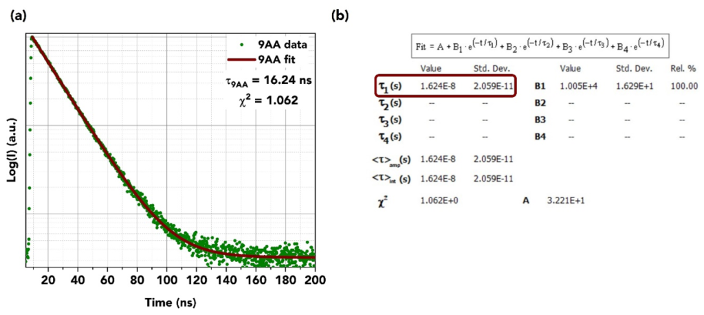
Figure 2. (a) Decay of 9AA measured using an FS5 Spectrofluorometer and (b) single exponential fit analysis in Fluoracle. 

Example Single Component Result

Here, τ is determined by tail fitting a single exponential component to the measured decay in Fluoracle. Fluoracle adjusts the value of τ and B until the least squares fit with the lowest residuals is achieved, which is 16.2 ns for 9AA (Figure 2b).  

Fluoracle can also calculate the lifetime using the time it takes the intensity to reduce to 1/e which has the advantage of not requiring least squares fitting. The 1/e lifetime for the 9AA decay was 16.4 ns, close to the fitted value of 16.2 ns. For single exponential decays, the 1/e calculation provides a quick estimate of the lifetime, but this method cannot be applied to more complex decays.   

Untangling Multi-Exponential Decays

When a sample contains multiple fluorophores, or a single molecule has multiple fluorescent populations (e.g. conformers or tautomers), a multi-exponential model must be used:

Where I(t) is the fluorescence intensity as a function of time, t, normalised to the intensity at t = 0, τi is the fluorescence lifetime of the ith decay component and Bi is the component amplitude. 

In theory, there is no limit to the number of exponential components that can be included in the model but there is a practical limit before the model loses physical meaning. A ‘better’ fit can always be achieved by increasing the number of components but that does not mean it is sensible to do so. For the lifetime components to be meaningful they must represent distinct photophysical processes occurring in the sample and the number of components should therefore be chosen based on knowledge of the expected photophysics.   

An example of a multiexponential decay is from a thermally activated delayed fluorescence (TADF) dye. The characteristic biexponential behaviour of a TADF dye can be seen in Figure 3a. The decay can be accurately modelled with two exponential decay components, τ1 = 65 ns and τ2 = 1061 ns which correspond to prompt fluorescence and delayed (after reverse intersystem crossing from the T1) fluorescence from the S1 excited state of the dye. 

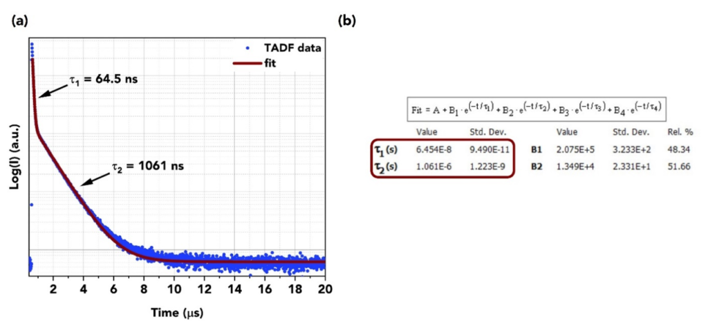
Figure 3. (a) A biexponential decay of TADF measured using the FS5 Spectrofluorometer and (b) fitting result in Fluoracle. 

Non-Exponential Decays

There are many sample types which do not follow exponential emission behaviour. This is often the case with photoluminescence decays from inorganic materials including semiconductors and ensemble emitters such as quantum dots. An example of a non-exponential decay is photoluminescence from indium phosphide quantum dots coated with a layer of zinc sulphide (InP/ZnS) shown in Figure 4.  

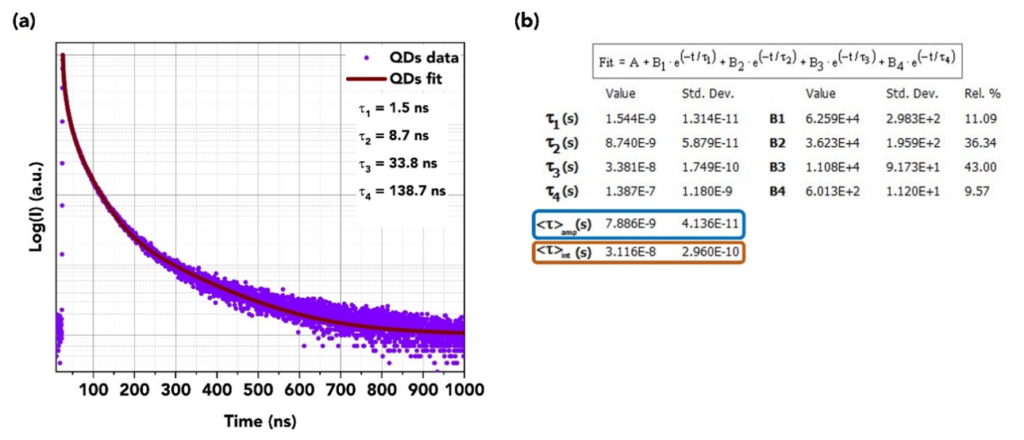
Figure 4. (a) Photoluminescence decay of InP/ZnS quantum dots measured using the FS5 Spectrofluorometer and (b) the corresponding fit analysis in Fluoracle with the amplitude weighted average lifetime (blue box) and the intensity weighted average lifetime (orange box) highlighted. 

A popular approach for this type of decay is to fit the decay with multiple exponential components and then calculate the average lifetime of the decay from the fit. This approach is shown in Figure 4a and 4b where Fluoracle has been used to fit the decay with four exponential components. The four individual lifetime components have no physical relation to specific states or interactions but are simply a means to fit the decay curve accurately. From the four lifetime components Fluoracle then calculates two average lifetime values, the amplitude weighted average lifetime and the intensity weighted average lifetime which can be used as a figure of merit to describe the photoluminescence lifetime properties of the sample. 

Average Lifetime 

Two average lifetimes are shown in Fluoracle as there is more than one definition of the average lifetime. The two average lifetimes most often reported in the literature are the amplitude weighted average lifetime and the intensity weighted average lifetime. Prior knowledge of the intrinsic mechanisms that lead to the depopulation of the material’s excited states is required to choose which average lifetime should be used. 

Amplitude Average Lifetime

The amplitude average lifetime, <τ>amp, weights each lifetime component (τi) by its amplitude (Bi):4 

where

The amplitude average lifetime is chara

cteristic of the fluorophore in the steady state and may be mathematically related to the rate constants.​3 ​The amplitude average lifetime is commonly used in biological systems where energy transfer between fluorophores occurs, and hence, their lifetime decay is multiexponential due to their heterogeneity and their interaction with their ambient environment.

It is worth noting that if the Bi component amplitudes are normalised (add up to 1) then the denominator in Eq. 7 becomes 1 and it therefore common to see Eq. 7 written as the numerator only. Fluoracle does not normalise the  Bi values and the full form of Eq. 7 is therefore used.

Intensity Average Lifetime 

The intensity average lifetime weights each lifetime component (τi) by the intensity of that component (Bi τi):4  

The intensity average places greater emphasis on the longer lifetimes, reducing the visibility of changes in fractional amplitude and shorter lifetimes. This makes the average appear more stable to changes in the number of components during fitting.​2 ​The intensity average lifetime is applicable in, e.g., an ensemble of emitters, such as quantum dots embedded in photonic crystals, and semiconductor nanocrystals whose fluorescence is nanocrystal size dependent.​5​ Nanocrystals of the same material but of different sizes will emit at different wavelengths and therefore, the average lifetime for the whole excited population of the nanocrystals should be considered. 

Knowing Your Samples 

Fits are best evaluated by careful evaluation of the photophysics of the chemical system, and the mathematically calculated ‘best’ solution is not always the correct answer. Fitting algorithms are blind to the system they are analysing. A single component rare-earth sample is treated in the same way as a non-exponential QD system. This means that the experimentalist should always make the final decision using sample-specific knowledge. Fitting is heavily shaped by the values input by the user (fitting range, background, suggested lifetimes). The fitting result is greatly affected by even small changes in these values, and these changes will have a non-calculable influence on the final fit.

Analysing Multiple Data Sets

This blog explores the basics of fitting for a single sample decay profile. To improve the understanding of a system multiple decay functions may be analysed together. A single sample may be measured with varied excitation or emission wavelength, or a series of samples with varying composition, will all have shared lifetimes. This can be linked using global fitting where multiple decay curves are fitted in parallel with some fitting parameters in common.   

References

1. D. M. Jameson, Introduction to Fluorescence, 2014. 

2. E. Fišerová and M. Kubala, Mean fluorescence lifetime and its error, J Lumin, 2012, 132, 2059–2064. 

3. A. Sillen and Y. Engelborghs, The Correct Use of ‘Average’ Fluorescence Parameters, Photochem Photobiol, 1998, 67, 475–486. 

4. B. Valeur and M. N. Berberan-Santos, Molecular Fluorescence, Wiley-VCH, 2nd edn., 2012. 

5. G. Zatryb and M. M. Klak, On the choice of proper average lifetime formula for an ensemble of emitters showing non-single exponential photoluminescence decay, Journal of Physics Condensed Matter, DOI:10.1088/1361-648X/ab9bcc.